In this chapter we introduce the definitions of two types of randomized algorithms: Monte Carlo algorithms and Las Vegas algorithms. The rest of the chapter is devoted to a case study: Monte Carlo algorithm for the minimum cut problem. The algorithm illustrates how a simple randomized algorithm can be powerful enough to solve a non-trivial problem. Furthermore, the analysis is quite elegant and uses some of the concepts we have learned in the last chapter. Finally, the algorithm allows us to present a very important and powerful technique: boosting the success probability of randomized algorithms by repeated trials.
Informally, we’ll say that an algorithm is randomized if it has access to a randomness source. In this course, we’ll assume that a randomized algorithm is allowed to call RandInt(\(m\)), which returns a uniformly random element of \(\{1,2,\ldots,m\}\), and Bernoulli(\(p\)), which returns \(1\) with probability \(p\) and returns \(0\) with probability \(1-p\). We assume that both RandInt and Bernoulli take \(O(1)\) time to execute. The notion of a randomized algorithm can be formally defined using probabilistic Turing machines, but we will not do so here.
Let \(f : \Sigma^* \to \Sigma^*\) be a computational problem. Let \(0 \leq \epsilon < 1\) be some parameter and \(T :\mathbb N\to \mathbb N\) be some function. Suppose \(A\) is a randomized algorithm such that
for all \(x \in \Sigma^*\), \(\Pr[A(x) \neq f(x)] \leq \epsilon\);
for all \(x \in \Sigma^*\), \(\Pr[\text{number of steps $A(x)$ takes is at most $T(|x|)$}] = 1\).
(Note that the probabilities are over the random choices made by \(A\).) Then we say that \(A\) is a \(T(n)\)-time Monte Carlo algorithm that computes \(f\) with \(\epsilon\) probability of error.
Let \(f : \Sigma^* \to \Sigma^*\) be a computational problem. Let \(T :\mathbb N\to \mathbb N\) be some function. Suppose \(A\) is a randomized algorithm such that
for all \(x \in \Sigma^*\), \(\Pr[A(x) = f(x)] = 1\), where the probability is over the random choices made by \(A\);
for all \(x \in \Sigma^*\), \(\mathbb{E}[\text{number of steps $A(x)$ takes}] \leq T(|x|)\).
Then we say that \(A\) is a \(T(n)\)-time Las Vegas algorithm that computes \(f\).
One can adapt the definitions above to define the notions of Monte Carlo algorithms and Las Vegas algorithms that compute decision problems (i.e. languages) and Monte Carlo algorithms and Las Vegas algorithms computing optimization problems (Definition (Optimization problem)).
Suppose you are given a Las Vegas algorithm \(A\) that solves \(f:\Sigma^* \to \Sigma^*\) in expected time \(T(n)\). Show that for any constant \(\epsilon > 0\), there is a Monte Carlo algorithm that solves \(f\) in time \(O(T(n))\) and error probability \(\epsilon\).
Given the Las Vegas algorithm \(A\) and a constant \(\epsilon > 0\), we construct a Monte Carlo algorithm \(A'\) with the desired properties as follows.
\[\begin{aligned} \hline\hline\\[-12pt] &\textbf{def}\;\; A'(x):\\ &{\scriptstyle 1.}~~~~\texttt{Run $A(x)$ for $\frac{1}{\epsilon}T(|x|)$ steps.}\\ &{\scriptstyle 2.}~~~~\texttt{If $A$ terminates, return its output.}\\ &{\scriptstyle 3.}~~~~\texttt{Else, return ``failure''.}\\ \hline\hline\end{aligned}\]
Since \(\epsilon\) is a constant, the running time of \(A'\) is \(O(T(n))\). The error probability of the algorithm can be bounded using Theorem (Markov’s inequality) as follows. For any \(x \in \Sigma^*\), let \(\mathbf{T}_x\) be the random variable that denotes the number of steps \(A(x)\) takes. Note that by Definition (Las Vegas algorithm), \(\mathbb{E}[\mathbf{T}_x] \leq T(|x|)\) for all \(x\). In the event of \(A'(x)\) failing, it must be the case that \(\mathbf{T}_x > \frac{1}{\epsilon} T(|x|)\). So the probability that \(A'(x)\) fails can be upper bounded by \[\Pr\left[\mathbf{T}_x > \frac{1}{\epsilon} T(|x|)\right] \leq \Pr\left[\mathbf{T}_x \geq \frac{1}{\epsilon} \mathbb{E}[\mathbf{T}_x]\right] \leq \epsilon,\] where the last inequality follows from Markov’s Inequality.
Technicality: There is a small technical issue here. Algorithm \(A'\) needs to be able to compute \(T(|x|)\) from \(x\) in \(O(T(|x|))\) time. This is indeed the case for most \(T(\cdot)\) that we care about.
Suppose you are given a Monte Carlo algorithm \(A\) that runs in worst-case \(T_1(n)\) time and solves \(f:\Sigma^* \to \Sigma^*\) with success probability at least \(p\) (i.e., for every input, the algorithm gives the correct answer with probability at least \(p\) and takes at most \(T_1(n)\) steps). Suppose it is possible to check in \(T_2(n)\) time whether the output produced by \(A\) is correct or not. Show how to convert \(A\) into a Las Vegas algorithm that runs in expected time \(O((T_1(n)+T_2(n))/p)\).
Given the Monte Carlo algorithm \(A\) as described in the question, we create a Las Vegas algorithm \(A'\) as follows.
\[\begin{aligned} \hline\hline\\[-12pt] &\textbf{def}\;\; A'(x):\\ &{\scriptstyle 1.}~~~~\texttt{Repeat:}\\ &{\scriptstyle 2.}~~~~~~~~\texttt{Run $A(x)$.}\\ &{\scriptstyle 3.}~~~~~~~~\texttt{If the output is correct, return the output.}\\ \hline\hline\end{aligned}\]
For all \(x\in \Sigma^*\), the algorithm gives the correct answer with probability 1.
For \(x \in \Sigma^*\), define \(\mathbf{T}_x\) to be the random variable corresponding to the number of iterations of the above algorithm. Observe that \(\mathbf{T}_x\) is a geometric random variable (Definition (Geometric random variable)) with success probability \(p\) (i.e., \(\mathbf{T}_x \sim \text{Geometric}(p)\)). The total number of steps \(A'(x)\) takes is thus \((T_1(|x|) + T_2(|x|)) \cdot \mathbf{T}_x\) (ignoring constant factors). The expectation of this value is \((T_1(|x|) + T_2(|x|)) \cdot \mathbb{E}[\mathbf{T}_x]\), where \(\mathbb{E}[\mathbf{T}_x] = 1/p\). So the total expected running time is \(O((T_1(|x|) + T_2(|x|))/p)\).
In the minimum cut problem, the input is a connected undirected graph \(G\), and the output is a \(2\)-coloring of the vertices, where each color is used at least once, such that the number of cut edges is minimized. (See Definition (Max-cut problem) for the definition of a cut edge.) Equivalently, we want to output a non-empty subset \(S \subsetneq V\) such that the number of edges between \(S\) and \(V\backslash S\) is minimized. Such a set \(S\) is called a cut and the size of the cut is the number of edges between \(S\) and \(V\backslash S\) (note that the size of the cut is not the number of vertices). We denote this problem by \(\text{MIN-CUT}\).
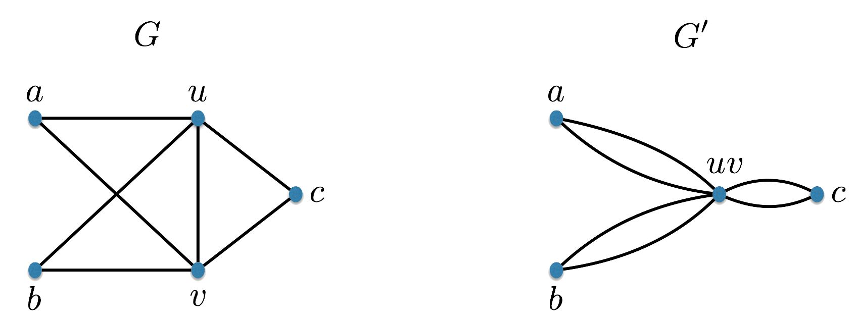
Let \(G=(V,E)\) be a multi-graph and let \(u,v \in V\) be two vertices in the graph. Contraction of \(u\) and \(v\) produces a new multi-graph \(G'=(V',E')\). Informally, in \(G'\), we collapse/contract the vertices \(u\) and \(v\) into one vertex and preserve the edges between these two vertices and the other vertices in the graph. Formally, we remove the vertices \(u\) and \(v\), and create a new vertex called \(uv\), i.e. \(V' = V \backslash \{u,v\} \cup \{uv\}\). The multi-set of edges \(E'\) is defined as follows:
for each \(\{u,w\} \in E\) with \(w \neq v\), we add \(\{uv,w\}\) to \(E'\);
for each \(\{v,w\} \in E\) with \(w \neq u\), we add \(\{uv,w\}\) to \(E'\);
for each \(\{w,w'\} \in E\) with \(w,w' \not \in \{u,v\}\), we add \(\{w,w'\}\) to \(E'\).
Below is an example:

There is a polynomial-time Monte-Carlo algorithm that solves the MIN-CUT problem with error probability at most \(1/e^n\), where \(n\) is the number of vertices in the input graph.
The algorithm has two phases. The description of the first phase is as follows.
\[\begin{aligned} \hline\hline\\[-12pt] &\textbf{def}\;\; A(\langle \text{graph } G = (V,E) \rangle):\\ &{\scriptstyle 1.}~~~~\texttt{Repeat until two vertices remain:}\\ &{\scriptstyle 2.}~~~~~~~~\texttt{Select an edge $\{u,v\}$ uniformly at random.}\\ &{\scriptstyle 3.}~~~~~~~~\texttt{Update the graph by contracting $u$ and $v$.}\\ &{\scriptstyle 4.}~~~~\texttt{Two vertices remain, corresponding to a partition $(V_1,V_2)$ of $V$; return $V_1$.}\\ \hline\hline\end{aligned}\]
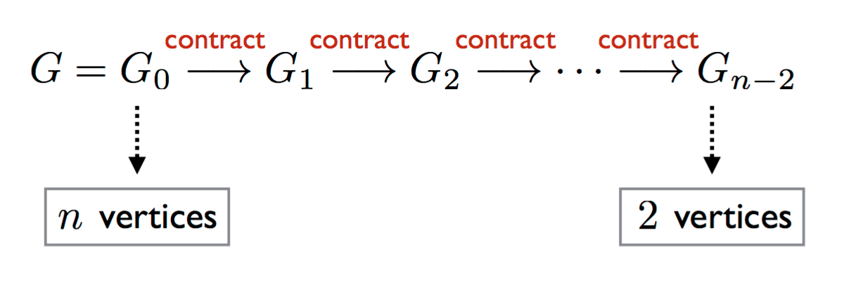
Let \(G_i\) denote the graph we have after \(i\) iterations of the algorithm. So \(G_0 = G\), \(G_1\) is the graph after we contract one of the edges, and so on. Note that the algorithm has \(n-2\) iterations because in each iteration the number of vertices goes down by exactly one and we stop when 2 vertices remain.

This makes it clear that the algorithm runs in polynomial time: we have \(n-2\) iterations, and in each iteration we can contract an edge, which can be done in polynomial time. Our goal now is to show that the success probability of the first phase, i.e., the probability that the above algorithm outputs a minimum cut, is at least \[\frac{2}{n(n-1)} \geq \frac{1}{n^2}.\] In the second phase, we’ll boost the success probability to the desired \(1 - 1/e^n\). We make two observations.
Observation 1: For any \(i\), a cut in \(G_i\) of size \(k\) corresponds to a cut in \(G = G_0\) of size \(k\). (We leave the proof of this as an exercise.)
Observation 2: For any \(i\) and any vertex \(v\) in \(G_i\), the size of the minimum cut (in \(G\)) is at most \(\deg_{G_i}(v)\). This is because a single vertex \(v\) forms a cut by itself (i.e. \(S=\{v\}\) is a cut), and the size of this cut is \(\deg(v)\). By Observation 1, the original graph \(G\) has a corresponding cut with the same size. Since the minimum cut has the minimum possible size among all cuts in \(G\), its size cannot be larger than \(\deg(v)\).
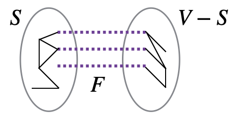
We are now ready to analyze the success probability of the first phase. Let \(F \subseteq E\) correspond to an optimum solution, i.e., a minimum size set of cut edges, with the corresponding partition of \(S\) and \(V \setminus S\).

We will show \[\Pr[\text{algorithm finds $F$}] \geq \frac{2}{n(n-1)}.\]
Let’s first observe that the algorithm’s output corresponds to \(F\) if and only if it never contracts an edge of \(F\). The argument for this observation is as follows. First, if the algorithm picks an edge in \(F\) to contract, that edge is removed, and so the output cannot correspond to \(F\). For the other direction, if the algorithm never contracts an edge in \(F\), then that means it only contracts edges within \(S\), or edges within \(V \setminus S\). The algorithm keeps contracting edges until two vertices remain, so this means all the vertices in \(S\) merge and become a single vertex, and all the vertices in \(V \setminus S\) merge and become a single vertex. That is when the algorithm stops and outputs the cut \(F\).
Now let \(E_i\) be the event that at iteration \(i\) of the algorithm, an edge in \(F\) is contracted. As noted above, there are \(n-2\) iterations in total. Therefore, \[\Pr[\text{algorithm finds $F$}] = \Pr[\overline{E}_1 \cap \overline{E}_2 \cap \ldots \cap \overline{E}_{n-2}].\] Using Proposition (Chain rule), we have \[\begin{gathered} \Pr[\overline{E}_1 \cap \overline{E}_2 \cap \ldots \cap \overline{E}_{n-2}] = \\ \Pr[\overline{E}_1] \cdot \Pr[\overline{E}_2 \; | \;\overline{E}_1] \cdot \Pr[\overline{E}_3 \; | \;\overline{E}_1 \cap \overline{E}_2] \cdots \Pr[\overline{E}_{n-2} \; | \;\overline{E}_1 \cap \overline{E}_2 \cap \ldots \cap \overline{E}_{n-3}]. \quad (*)\end{gathered}\] To lower bound the success probability of the algorithm, we’ll find a lower bound for each term of the RHS of the above equation. We start with \(\Pr[\overline{E}_1]\). It is easy to see that \(\Pr[E_1] = |F|/m\). However, it will be more convenient to have a bound on \(\Pr[E_1]\) in terms of \(|F|\) and \(n\) rather than \(m\). By Observation 2 above, we know \[\forall v \in V, \quad |F| \leq \deg(v).\] Using this, we have \[\begin{aligned} 2m = \sum_{v \in V} \deg(v) \geq |F|\cdot n, \quad \quad (**)\end{aligned}\] or equivalently, \(|F| \leq 2m/n\). Therefore, \[\Pr[E_1] = \frac{|F|}{m} \leq \frac{2}{n},\] or equivalently, \(\Pr[\overline{E}_1] \geq 1 - 2/n\). At this point, going back to Equality (*) above, we can write \[\begin{gathered} \Pr[\text{algorithm finds $F$}] \geq \\ \left(1 - \frac{2}{n}\right) \cdot \Pr[\overline{E}_2 \; | \;\overline{E}_1] \cdot \Pr[\overline{E}_3 \; | \;\overline{E}_1 \cap \overline{E}_2] \cdots \Pr[\overline{E}_{n-2} \; | \;\overline{E}_1 \cap \overline{E}_2 \cap \ldots \cap \overline{E}_{n-3}]. \end{gathered}\] We move onto the second term \(\Pr[\overline{E}_2 \; | \;\overline{E}_1]\). Let \(\ell_1\) be the number of edges remaining after the first iteration of the algorithm. Then \[\Pr[\overline{E}_2 \; | \;\overline{E}_1] = 1 - \Pr[E_2 \; | \;\overline{E}_1] = 1 - \frac{|F|}{\ell_1}.\] As before, using Observation 2, for any \(v\) in \(G_1\), \(|F| \leq \deg_{G_1}(v)\). Therefore, the analog of Inequality (**) above for the graph \(G_1\) yields \(2\ell_1 \geq |F|(n-1)\). Using this inequality, \[\Pr[\overline{E}_2 \; | \;\overline{E}_1] = 1 - \frac{|F|}{\ell_1} \geq 1 - \frac{2|F|}{|F|(n-1)} = 1 - \frac{2}{n-1}.\] Thus \[\begin{gathered} \Pr[\text{algorithm finds $F$}] \geq \\ \left(1 - \frac{2}{n}\right) \cdot \left(1 - \frac{2}{n-1}\right) \cdot \Pr[\overline{E}_3 \; | \;\overline{E}_1 \cap \overline{E}_2] \cdots \Pr[\overline{E}_{n-2} \; | \;\overline{E}_1 \cap \overline{E}_2 \cap \ldots \cap \overline{E}_{n-3}]. \end{gathered}\] Applying the same reasoning for the rest of the terms in the product above, we get \[\begin{aligned} & \Pr[\text{algorithm finds $F$}] \geq \\ & \qquad \left(1 - \frac{2}{n}\right) \cdot \left(1 - \frac{2}{n-1}\right) \cdot \left(1 - \frac{2}{n-2}\right) \cdots \left(1 - \frac{2}{n-(n-3)}\right) = \\ & \qquad \left(\frac{n-2}{n} \right) \cdot \left(\frac{n-3}{n-1} \right) \cdot \left(\frac{n-4}{n-2} \right) \cdots \left(\frac{2}{4} \right) \cdot \left(\frac{1}{3} \right). \end{aligned}\] After cancellations between the numerators and denominators of the fractions, the first two denominators and the last two numerators survive, and the above simplifies to \(2/n(n-1)\). So we have reached our goal for the first phase and have shown that \[\Pr[\text{algorithm finds $F$}] \geq \frac{2}{n(n-1)} = \frac{1}{{n \choose 2}} \geq \frac{1}{n^2}.\] This implies \[\Pr[\text{algorithm finds a min-cut}] \geq \frac{1}{n^2}.\]
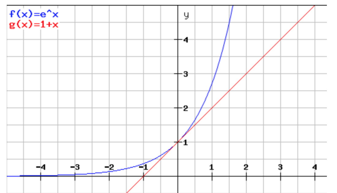
In the second phase of the algorithm, we boost the success probability by repeating the first phase \(t\) times using completely new and independent random choices. Among the \(t\) cuts we find, we return the minimum-sized one. As \(t\) grows, the success probability increases. Our analysis will show that \(t = n^3\) is sufficient for the bound we want. Let \(A_i\) be the event that our algorithm does not find a min-cut at repetition \(i\). Note that the \(A_i\)’s are independent since our algorithm uses fresh random bits for each repetition. Also, each \(A_i\) has the same probability, i.e. \(\Pr[A_i] = \Pr[A_j]\) for all \(i\) and \(j\). Therefore, \[\begin{aligned} \Pr[\text{our algorithm fails to find a min-cut}] & = \Pr[A_1\cap \cdots \cap A_t] \\ & = \Pr[A_1] \cdots \Pr[A_t] \\ & = \Pr[A_1]^t.\end{aligned}\] From the analysis of the first phase, we know that \[\Pr[A_1] \leq 1 - \frac{1}{n^2}.\] So \[\Pr[\text{our algorithm fails to find a min-cut}] \leq \left(1 - \frac{1}{n^2}\right)^t.\] To upper bound this, we’ll use an extremely useful inequality: \[\forall x \in \mathbb{R}, \quad 1+x \leq e^x.\] We will not prove this inequality, but we provide a plot of the two functions below.

Notice that the inequality is close to being tight for values of \(x\) close to \(0\). Letting \(x = -1/n^2\), we see that \[\Pr[\text{our algorithm fails to find a min-cut}] \leq (1 + x)^t \leq e^{xt} = e^{-t/n^2}.\] For \(t = n^3\), this probability is upper bounded by \(1/e^n\), as desired.
This question asks you to boost the success probability of a Monte Carlo algorithm computing a decision problem with one-sided error.
Let \(f:\Sigma^* \to \{0,1\}\) be a decision problem, and let \(A\) be a Monte Carlo algorithm for \(f\) such that if \(x\) is a YES instance, then \(A\) always gives the correct answer, and if \(x\) is a NO instance, then \(A\) gives the correct answer with probability at least 1/2. Suppose \(A\) runs in worst-case \(O(T(n))\) time. Design a new Monte Carlo algorithm \(A'\) for \(f\) that runs in \(O(nT(n))\) time and has error probability at most \(1/2^n\).
Here is the description of \(A'\).
\[\begin{aligned} \hline\hline\\[-12pt] &\textbf{def}\;\; A'(x):\\ &{\scriptstyle 1.}~~~~\texttt{Repeat $|x|$ times:}\\ &{\scriptstyle 2.}~~~~~~~~\texttt{Run $A(x)$.}\\ &{\scriptstyle 3.}~~~~~~~~\texttt{If the output is $0$, return $0$.}\\ &{\scriptstyle 4.}~~~~\texttt{Return $1$.}\\ \hline\hline\end{aligned}\]
We call \(A(x)\) \(n\) times, and the running time of \(A\) is \(O(T(n))\), so the overall running time of \(A'\) is \(O(nT(n))\).
To prove the required correctness guarantee, we need to show that for all inputs \(x\), \(\Pr[A'(x) \neq f(x)] \leq 1/2^n\). For any \(x\) such that \(f(x) = 1\), we know that \(\Pr[A(x) = 1] = 1\), and therefore \(\Pr[A'(x) = 1] = 1\). For any \(x\) such that \(f(x) = 0\), we know that \(\Pr[A(x) = 0] \geq 1/2\). The only way \(A'\) makes an error in this case is if \(A(x)\) returns 1 in each of the \(n\) iterations. So if \(E_i\) is the event that in iteration \(i\), \(A(x)\) returns the wrong answer (i.e. returns 1), we are interested in upper bounding \(\Pr[\text{error}] = \Pr[E_1 \cap E_2 \cap \cdots \cap E_n]\). Note that the \(E_i\)’s are independent (one run of \(A(x)\) has no effect on other runs of \(A(x)\)). Furthermore, for all \(i\), \(\Pr[E_i] \leq 1/2\). So \[\Pr[E_1 \cap E_2 \cap \cdots \cap E_n] = \Pr[E_1] \Pr[E_2] \cdots \Pr[E_n] \leq 1/2^n,\] as desired.
This question asks you to boost the success probability of a Monte Carlo algorithm computing a decision problem with two-sided error.
Let \(f:\Sigma^* \to \{0,1\}\) be a decision problem, and let \(A\) be a Monte Carlo algorithm for \(f\) with error probability \(1/4\), i.e., for all \(x \in \Sigma^*\), \(\Pr[A(x) \neq f(x)] \leq 1/4\). We want to boost the success probability to \(1-1/2^n\), and our strategy will be as follows. Given \(x\), run \(A(x)\) \(6n\) times (where \(n = |x|\)), and output the more common output bit among the \(6n\) output bits (breaking ties arbitrarily). Show that the probability of outputting the wrong answer is at most \(1/2^n\).
Let \(\mathbf{X}_i\) be a Bernoulli random variable corresponding to whether the algorithm gives the correct answer in iteration \(i\). That is, \[\mathbf{X}_i = \begin{cases} 1 & \text{ if algorithm gives correct answer in iteration $i$,}\\ 0 & \text{ otherwise.} \end{cases}\] Let \(\mathbf{X} = \sum_{i=1}^{6n} \mathbf{X}_i\). So \(\mathbf{X} \sim \text{Bin}(6n, 3/4)\) (see Definition (Binomial random variable)). Note that \[\Pr[\mathbf{X} = i] = {6n \choose i} \left(\frac{3}{4}\right)^{i} \left(\frac{1}{4}\right)^{6n-i}.\] The algorithm is run \(6n\) times and we take the majority answer, so we make a mistake only if it was correct at most \(3n\) times, i.e. \(\Pr[\text{error}] \leq \Pr[\mathbf{X} \leq 3n]\), and so \[\Pr[\text{error}] \leq \sum_{i = 0}^{3n} \Pr[\mathbf{X} = i] = \sum_{i = 0}^{3n} {6n \choose i} \left(\frac{3}{4}\right)^{i} \left(\frac{1}{4}\right)^{6n-i}.\] We simplify the right-hand-side as follows. \[\begin{aligned} \sum_{i = 0}^{3n} {6n \choose i} \left(\frac{3}{4}\right)^{i} \left(\frac{1}{4}\right)^{6n-i} & = \sum_{i = 0}^{3n} {6n \choose i} \frac{3^i}{4^{6n}} \\ & \leq \sum_{i = 0}^{3n} {6n \choose i} \frac{3^{3n}}{4^{6n}} \\ & = \frac{3^{3n}}{4^{6n}} \cdot \sum_{i = 0}^{3n} {6n \choose i} \\ & \leq \frac{3^{3n}}{4^{6n}} \cdot 2^{6n} \\ & = \frac{27^n}{64^n} < \frac{1}{2^n}. \end{aligned}\]
Using the analysis of the randomized minimum cut algorithm, show that a graph can have at most \(n(n-1)/2\) distinct minimum cuts.
Suppose there are \(t\) distinct minimum cuts \(F_1, F_2, \ldots F_t\). Our goal is to show \(t \leq {n \choose 2}\). Let \(A_i\) be the event that the first phase of our algorithm in the proof of Theorem (Contraction algorithm for min cut) outputs \(F_i\) (the first phase refers to the phase before the boosting). We know that for any \(i\), \(\Pr[A_i] \geq 1/{n \choose 2}\) (as shown in the proof). Furthermore, the events \(A_i\) are disjoint (if one happens, another cannot happen). So \[\Pr[A_1 \cup A_2 \cup \cdots \cup A_t] = \Pr[A_1] + \Pr[A_2] + \cdots + \Pr[A_t] \geq \frac{t}{{n \choose 2}}.\] Since \(\Pr[A_1 \cup A_2 \cup \cdots \cup A_t] \leq 1\), we can conclude \[t \leq {n \choose 2}.\]
Suppose we modify the min-cut algorithm seen in lecture so that rather than picking an edge uniformly at random, we pick 2 vertices uniformly at random and contract them into a single vertex. True or False: The success probability of the algorithm (excluding the part that boosts the success probability) is \(1/n^k\) for some constant \(k\), where \(n\) is the number of vertices. Justify your answer.
If the success probability of a randomized algorithm is \(1/n^k\), that means that for all inputs, the probability that the algorithm gives the desired output is at least \(1/n^k\). So to show that the success probability cannot be \(1/n^k\), it suffices to present one input for which the success probability is smaller than \(1/n^k\) (e.g. exponentially small).
Let \(A\) and \(B\) be cliques of size \(n/2\) each. Join them together by a single edge to form the graph \(G\). Then the minimum cut is \(S = A\) with the single edge connecting \(A\) and \(B\) being the cut edge. Observe that the algorithm will output this cut if and only if it never picks vertices \(a \in A\) and \(b \in B\) to contract. The probability that the algorithm never picks \(a \in A\) and \(b \in B\) to contract is exponentially small. (We leave this part to the reader. Note that all you need is a bound; you do not have to calculate the probability exactly.)
True or false: When analyzing a randomized algorithm, we assume that the input is chosen uniformly at random.
What is the difference between a Monte Carlo algorithm and a Las Vegas algorithm?
Describe the probability tree induced by a Monte Carlo algorithm on a given input.
Describe the probability tree induced by a Las Vegas algorithm on a given input.
Describe at a high level how to convert a Las Vegas algorithm into a Monte Carlo algorithm.
Describe at a high level how to covert a Monte Carlo algorithm into a Las Vegas algorithm.
In this chapter, we defined the MIN-CUT problem. In the MAX-CUT problem, given a graph \(G=(V,E)\), we want to output a non-empty subset \(S \subsetneq V\) such that the number of edges between \(S\) and \(V\backslash S\) is maximized. Suppose for every vertex \(v \in V\), we flip a fair coin and put the vertex in \(S\) if the coin comes up heads. Show that the expected number of cut edges is \(|E|/2\).
Argue, using the result from previous question, why every graph with \(|E|\) edges contains a cut of size at least \(|E|/2\).
Outline a general strategy for boosting the success probability of a Monte Carlo algorithm that computes a decision problem.
True or false: For any decision problem, there is a polynomial-time Monte Carlo algorithm that computes it with error probability equal to \(1/2\).
Suppose we have a Monte-Carlo algorithm for a decision problem with error probability equal to \(1/2\). Can we boost the success probability of this algorithm by repeated trials?
True or false: The cut output by the contraction algorithm is uniformly random among all possible cuts.
True or false: The size of a minimum cut in a graph is equal to the minimum degree of a vertex in the graph.
Give an example of a problem for which we have a polynomial-time randomized algorithm, but we do not know of a polynomial-time deterministic algorithm.
As always, understanding the definitions is important. Make sure you are comfortable with the definitions of Monte Carlo and Las Vegas algorithms.
We require worst-case guarantees for randomized algorithms. In particular, in this course, we never consider a randomly chosen input.
One of the best ways to understand randomized algorithms is to have a clear understanding on how they induce a probability tree and what properties those probability trees have. We have emphasized this point of view in lecture even though it does not appear in this chapter.
It is important to know how to convert a Monte Carlo algorithm into a Las Vegas algorithm and vice versa.
The main example in this chapter is the analysis of the contraction algorithm for MIN-CUT. There are several interesting ideas in the analysis, and you should make note of those ideas/tricks. Especially the idea of boosting the success probability of a randomized algorithm via repeated trials is important.
One extremely useful trick that was highlighted in the previous chapter is the calculation of an expectation of a random variable by writing it as a sum of indicator random variables and using linearity of expectation (see Important Note (Combining linearity of expectation and indicators) and the exercise after it). This trick comes up a lot in the context of randomized algorithms. In particular, you will very likely be asked a question of the form “Give a randomized algorithm for problem X with the property that the expected number of Y is equal to Z.” As an example, see the analysis of the randomized algorithm for MAX-CUT problem covered in lecture.